Blue Noise Plots

Computer Graphics Forum (Proc. of Annual Conference of the European Association for Computer Graphics) 2021

Abstract

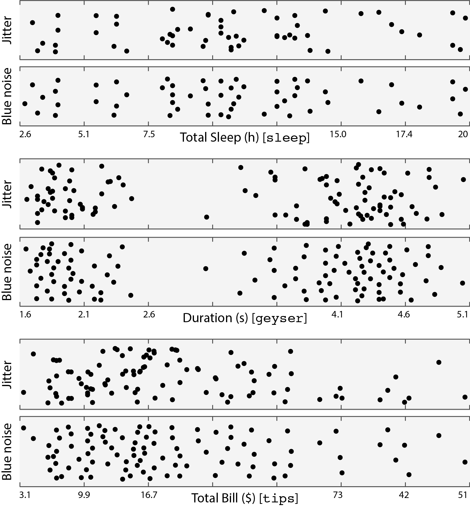
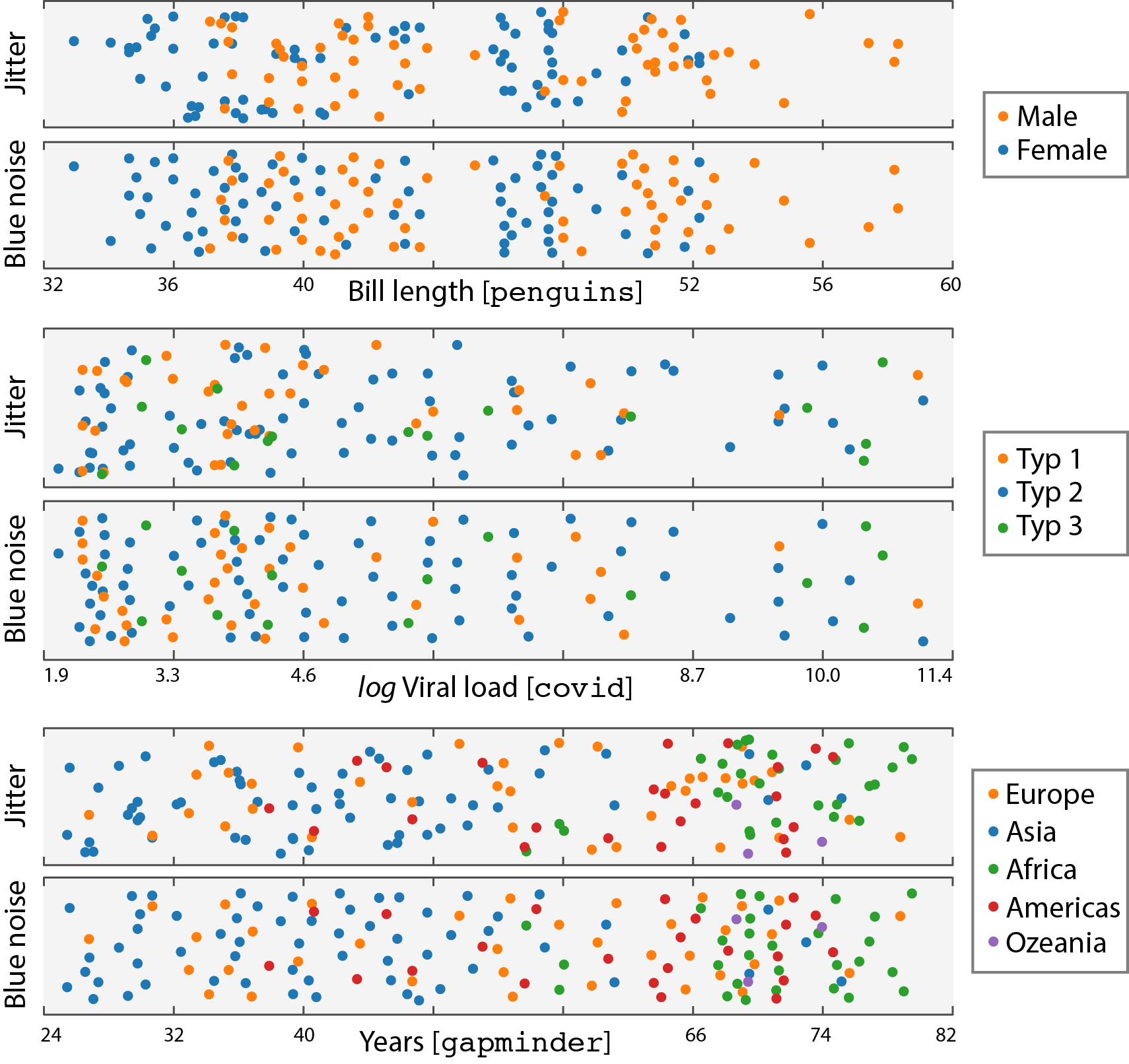
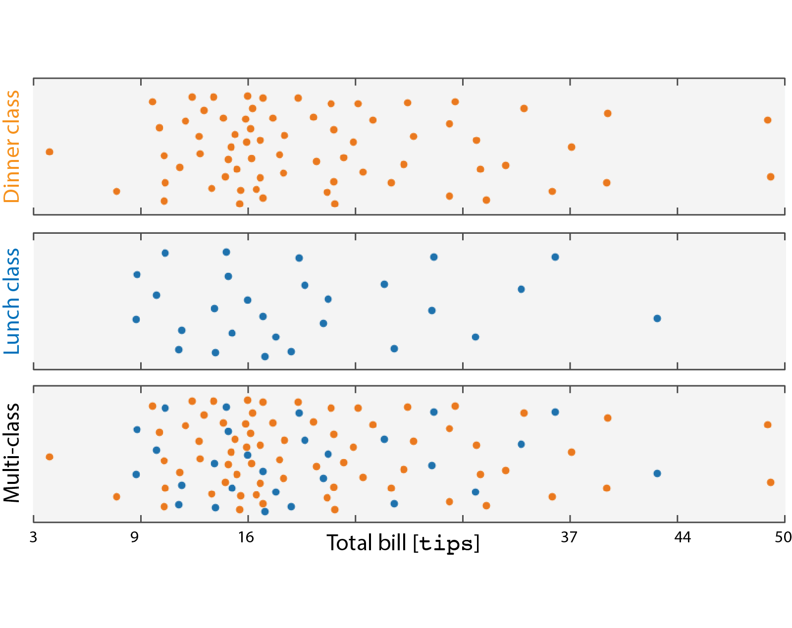
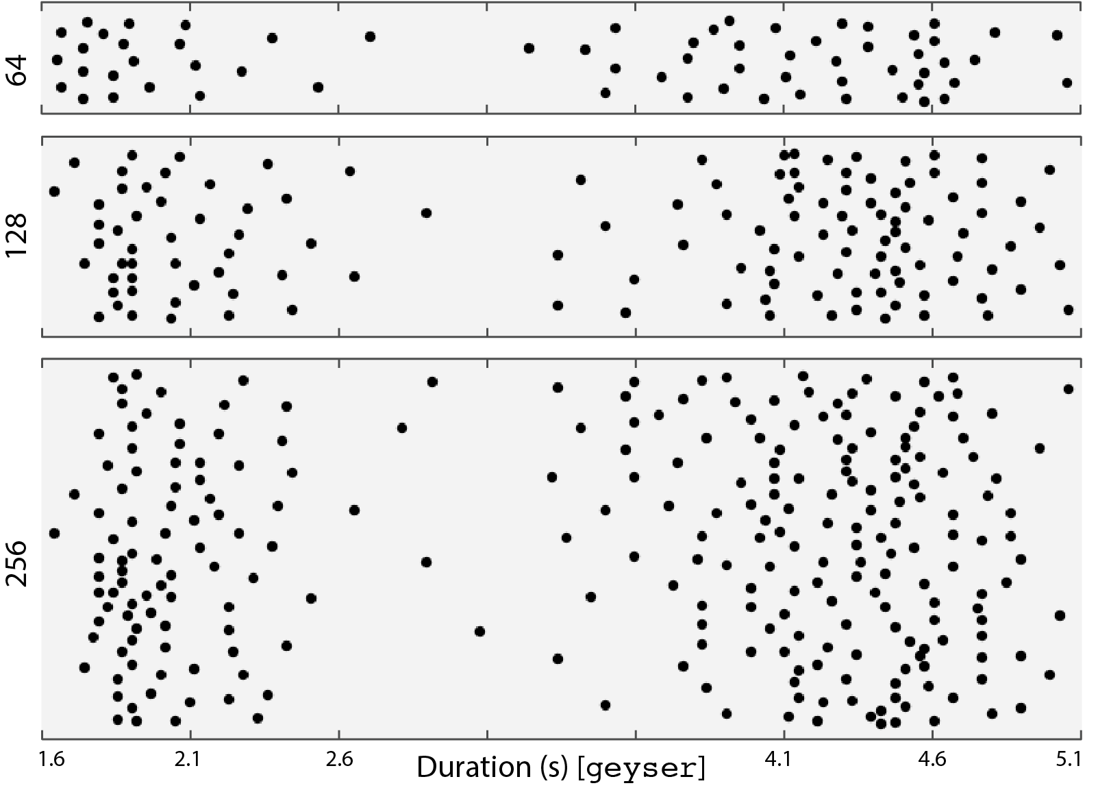
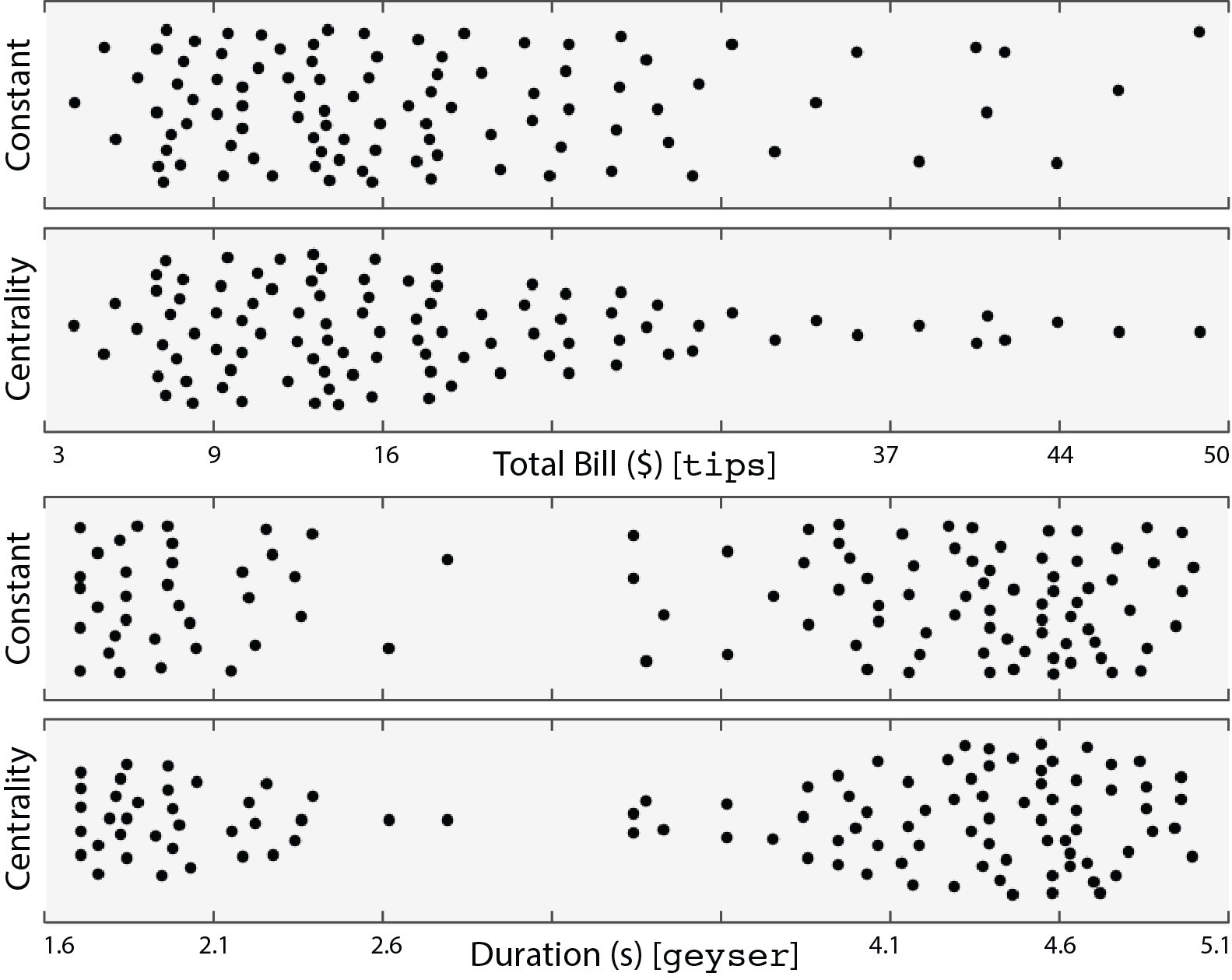
We propose Blue Noise Plots, two-dimensional dot plots that depict data points of univariate data sets. While often one-dimensional strip plots are used to depict such data, one of their main problems is visual clutter which results from overlap. To reduce this overlap, jitter plots were introduced, whereby an additional, non-encoding plot dimension is introduced, along which the data point representing dots are randomly perturbed. Unfortunately, this randomness can suggest non-existent clusters, and often leads to visually unappealing plots, in which overlap might still occur. To overcome these shortcomings, we introduce BlueNoise Plots where random jitter along the non-encoding plot dimension is replaced by optimizing all dots to keep a minimum distance in 2D i. e., Blue Noise. We evaluate the effectiveness as well as the aesthetics of Blue Noise Plots through both, a quantitative and a qualitative user study.

Bibtex

@article{vanOnzenoodt2021blue,
	title={Blue Noise Plots},
	author={van Onzenoodt, Christian and Singh, Gurprit and Ropinski, Timo and Ritschel, Tobias},
	year={2021},
	journal={Computer Graphics Forum (Proc. of Annual Conference of the European Association for Computer Graphics (2021))},
	volume={40},
	issue={2},
	doi={10.1111/cgf.142644}
}

Figures

Figure: Comparison of three different data sets, each of them visualized using a traditional jitter plot and our Blue Noise Plot.

Figure: Different examples of multi-class data sets, visualized using jitter plots as well as Blue Noise Plots.

Figure: Multi-class Blue Noise Plot for the tips data set withtwo classes: dinner and lunch encoded into color.

Figure: Comparison of adaptive plots with different numbers of dots. These plots show a random subset of the geyser data set, visualized using our Blue Noise Plot. Here a) shows 64 dots, b) shows 128 dots and finally c) shows 256 dots.

Figure: Optimal constant plot height (first and third) and a varying height (second and fourth), both for Blue Noise Plots.